Part 6 : Non-linear classification with Pytorch

In a previous post, we implemented from scratch a neural network to perform binary classification. The derivation of the equation and the calculation of the gradients become very quickly complex when the number of layers and neurons increases. In practice, we use deep learning libraries for that. In this example, we will implement the network seen previously using the Pytorch library.

Network architecture

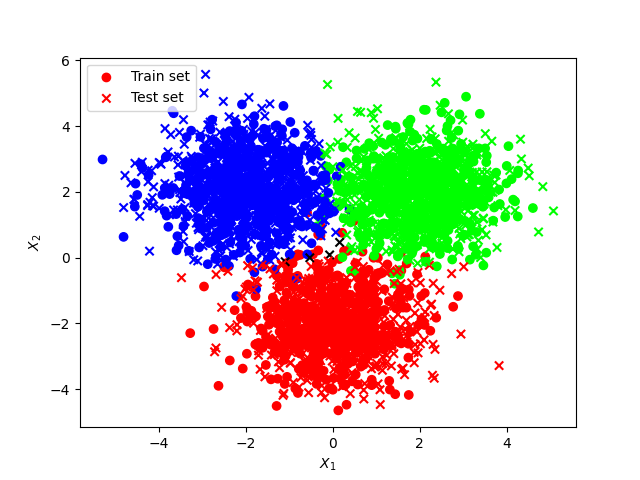
The data set and network architecture remains the same as in the previous post. i.e. A train set of 500 observations with a non-linear decision boundary. Each observations has 2 features (X1 and X2).

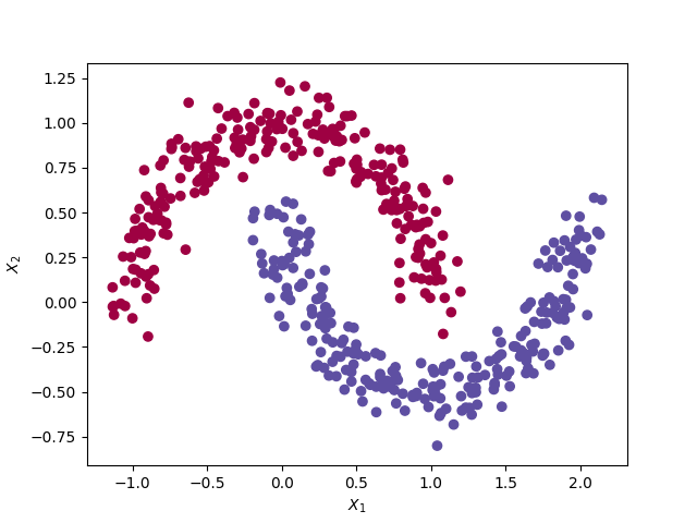_{^{The moon dataset from the Sklearn library}}

We choose an input layer of 2 neurons (since we have 2 features), a hidden layer of 4 neurons and an output layer of 1 neuron, which can take the value 0 or 1. The architecture of the network is as follows.

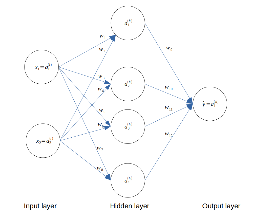_{^{Architecture of the neural network}}

Implementation

We start by importing the required libraries.

from sklearn.datasets import make_moons
from sklearn.preprocessing import StandardScaler   
from matplotlib.colors import ListedColormap
import numpy as np
import matplotlib.pyplot as plt
import torch
import torch.nn as nn

We create a training and testing set using the make_moons function from Scikit-Learn library. Note that we are need to normalise and transform our Numpy arrays to tensors.

def create_dataset(seed_nb):
    np.random.seed(seed_nb)
    X, y = make_moons(500, noise=0.10)  

    # Standardize the input
    scaler = StandardScaler()
    X = scaler.fit_transform(X)

    # Transform to tensor
    X = torch.from_numpy(X).type(torch.FloatTensor)
    y = torch.from_numpy(y).type(torch.FloatTensor)

    # Reshape y
    new_shape = (len(y), 1)
    y = y.view(new_shape)

    return X, y

X, y = create_dataset(seed_nb=4564)
X_test, y_test = create_dataset(seed_nb=8472)

We choose the same learning rate and number of epochs as in the precedent post.

alpha = 0.5  # learning rate
nb_epoch = 5000

We define our network based on the architecture. We will use the Sigmoid and MSE cost function as previously.

class Net(nn.Module):
    def __init__(self):
        super(Net, self).__init__()
        self.L0 = nn.Linear(2, 4)
        self.N0 = nn.Sigmoid()
        self.L1 = nn.Linear(4, 1)

    def forward(self, x):
        x = self.L0(x)
        x = self.N0(x)
        x = self.L1(x)
        return x
    
    def predict(self, x):
        return self.forward(x)

model = Net()
criterion = nn.MSELoss()
optimizer = torch.optim.Adam(model.parameters(), lr=alpha)
print(model)

This is how we train our network. Pytorch computes the gradients automatically.

costs = []

for epoch in range(nb_epoch):
    
    # Feedforward
    y_pred = model.forward(X)
    cost = criterion(y_pred, y)
    costs.append(cost.item())

    # Backpropagation
    optimizer.zero_grad()
    cost.backward()
    optimizer.step()
    
    if epoch % (nb_epoch // 100) == 0:
        print("Epoch {}/{} | cost function: {:.3f}".format(epoch, nb_epoch, cost.item()))

We can plot the evolution of the cost function with the number of epochs.

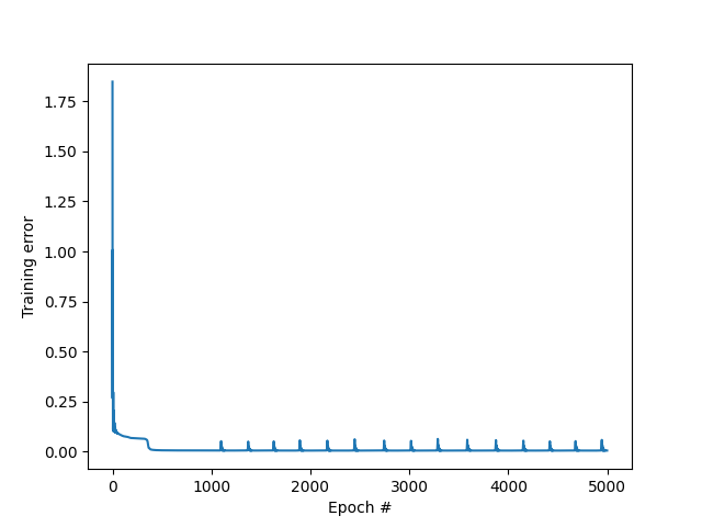_{^{MSE vs epoch}}

Finally, we test our network on the test set.

y_pred_test = model.predict(X_test)
y_pred_test = torch.round(y_pred_test)
cost_test = criterion(y_pred_test, y)

print('Train error final: ', cost.item())
print('Test error final: ', cost_test.item())

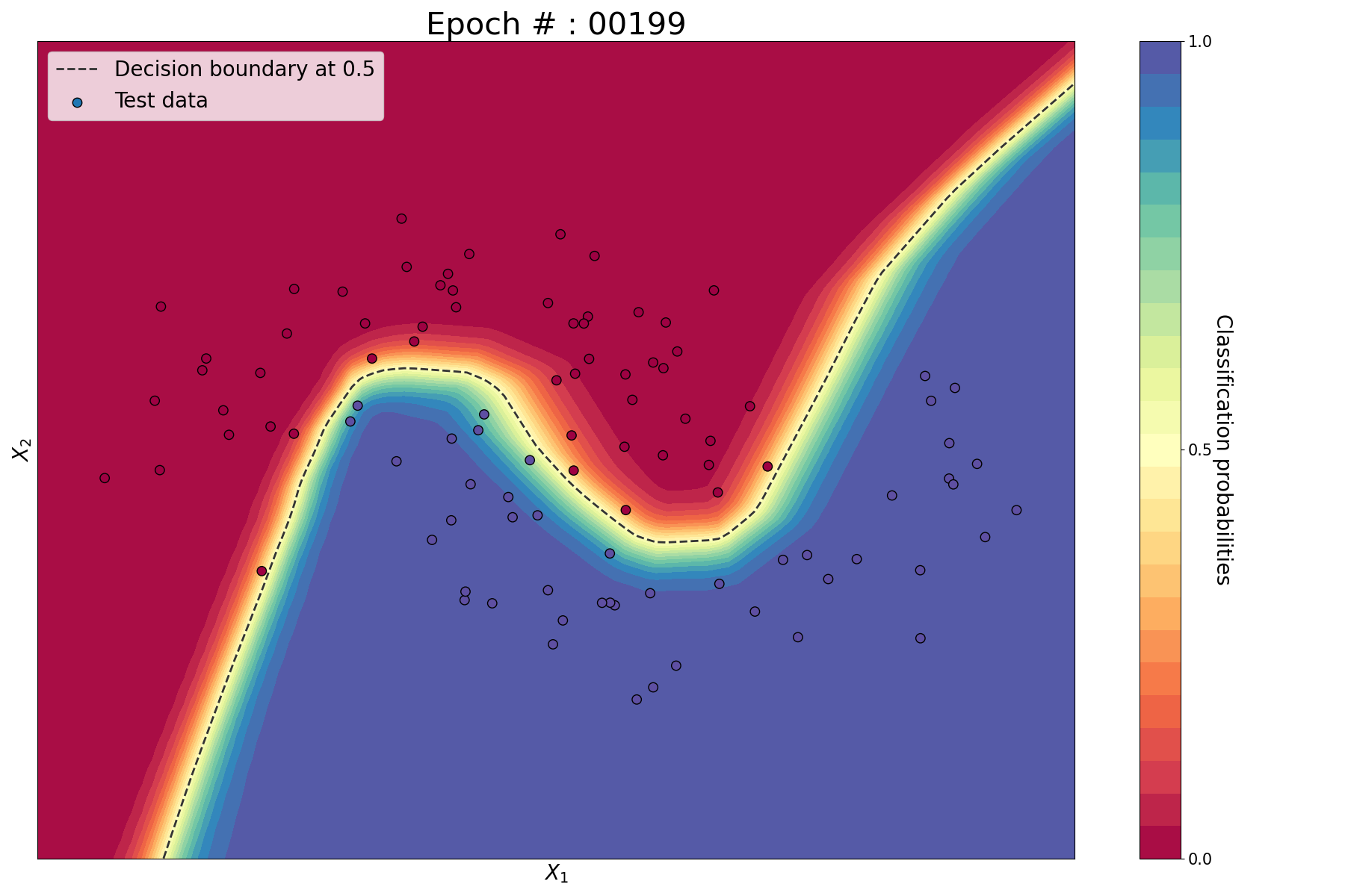
Since we are considering 2 features, we can conveniently plot the train set, test set, prediction probabilities and decision functions in 2D. For that, we implement the following helper function.

def predict(x):
    x = torch.from_numpy(x).type(torch.FloatTensor)
    ans = model.predict(x)
    return ans.detach().numpy()

def plot_decision_boundary(pred_func, X_train, y_train, X_test, y_test):

    # Define mesh grid
    h = .02
    x_min, x_max = X[:, 0].min() - .5, X[:, 0].max() + .5
    y_min, y_max = X[:, 1].min() - .5, X[:, 1].max() + .5

    xx, yy = np.meshgrid(np.arange(x_min, x_max, h),
                        np.arange(y_min, y_max, h))

    # Predict the function value for the whole grid
    Z = pred_func(np.c_[xx.ravel(), yy.ravel()])
    Z = Z.reshape(xx.shape)

    # Define figure and colormap
    fig, ax = plt.subplots(figsize=(10, 10))
    cm = plt.cm.viridis
    first, last = cm.colors[0], cm.colors[-1]
    cm_bright = ListedColormap([first, last])

    # Plot the contour, decision boundary, test and train data
    cb = ax.contourf(xx, yy, Z, levels=10, cmap=cm, alpha=0.8)
    CS = ax.contour(xx, yy, Z, levels=[.5], colors='k', linestyles='dashed', linewidths=2)
    ax.scatter(X_train[:, 0], X_train[:, 1], c=y_train, cmap=cm_bright, edgecolors='k', marker='o', s=100, linewidth=2, label="Train data")
    ax.scatter(X_test[:, 0], X_test[:, 1], c=y_test, cmap=cm_bright, edgecolors='k',marker='^', s=100, linewidth=2, label="Test data")

    # Colourbar, axis, title, legend
    fs = 15
    plt.clabel(CS, inline=1, fontsize=fs)
    CS.collections[0].set_label("Decision boundary at 0.5")
    plt.colorbar(cb, ticks=[0, 1])
    ax.legend(fontsize=fs, loc='upper left')
    ax.set_xlim(xx.min(), xx.max())
    ax.set_ylim(yy.min(), yy.max())
    ax.set_xlabel("$X_1$", fontsize=fs)
    ax.set_ylabel("$X_2$", fontsize=fs)
    ax.set_xticks(())
    ax.set_yticks(())


plot_decision_boundary(lambda x : predict(x), X.numpy(), y.numpy(), X_test.numpy(), y_test.numpy())
plt.tight_layout()
plt.savefig('plots/4_train_vs_test.png')
plt.show()

_{^{Train vs test set}}

You can find the code on my Github.

Conclusion

We used the Pytorch library to implement the neural network that we implemented from scratch previously.